분류(Classification)
[참조] 패스트캠퍼스 - 직장인을 위한 파이썬 데이터분석 올인원 패키지 Online.
iris 데이터셋
데이터셋 로드
from sklearn.datasets import load_iris
iris = load_iris()
Key 값
- DESCR: 데이터셋의 정보
- data: feature data
- feature_names: feature data의 컬럼 이름
- target: label data (수치형)
- target_names: label 이름 (문자형)
print(iris['DESCR'])
이처럼 원하는 Key 값을 넣어 확인이 가능하다.
데이터 프레임 생성
df_iris = pd.DataFrame(data, columns=feature_names)
df_iris['target'] = target
시각화
sns.scatterplot(x='sepal width (cm)', y='sepal length (cm)', hue='target', palette='muted', data=df_iris)
plt.title('Sepal')
plt.show()
- sepal(꽃 받침) 길이와 너비에 따른 분포도 확인
sns.scatterplot('petal width (cm)', 'petal length (cm)', hue='target', palette='muted', data=df_iris)
plt.title('Petal')
plt.show()
- petal(꽃잎) 길이와 너비에 따른 분포도 확인
from mpl_toolkits.mplot3d import Axes3D
from sklearn.decomposition import PCA

fig = plt.figure(figsize=(8, 6))
ax = fig.add_subplot(111, projection='3d')
X_reduced = PCA(n_components=3).fit_transform(df_iris.drop('target', 1))
ax.scatter(X_reduced[:, 0], X_reduced[:, 1], X_reduced[:, 2], c=df_iris['target'],
           cmap=plt.cm.Set1, edgecolor='k', s=40)
ax.set_title("Iris 3D")
ax.set_xlabel("x")
ax.w_xaxis.set_ticklabels([])
ax.set_ylabel("y")
ax.w_yaxis.set_ticklabels([])
ax.set_zlabel("z")
ax.w_zaxis.set_ticklabels([])

plt.show()
- 3D로 그래프를 그려 보여줄 수도 있다.
데이터 분류
from sklearn.model_selection import train_test_split
train_test_split로드
x_train, x_valid, y_train, y_valid = train_test_split(df_iris.drop('target', 1), df_iris['target'])
train_test_split()메서드에 인자 전달- 첫 번째 인자: feature 데이터
- 두 번째 인자: target 데이터
sns.countplot(x=y_train)
y_train에 대해 그래프를 그려보면 다음과 같이 보인다.
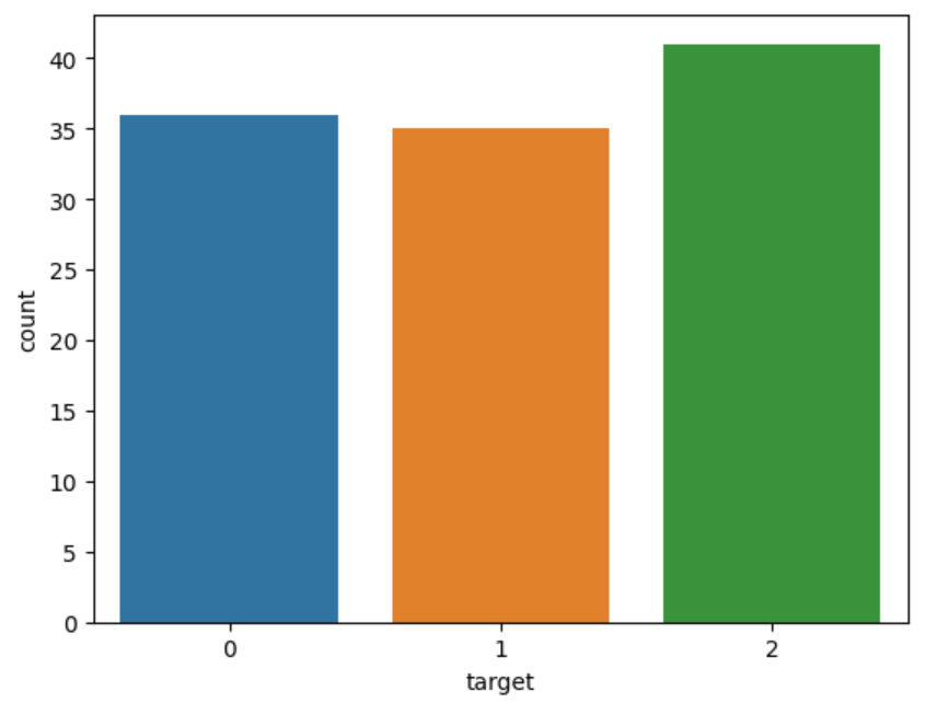
2번이 다른 데이터보다 많기 떄문에 2번에 편향된 학습이 진행될 수가 있다.
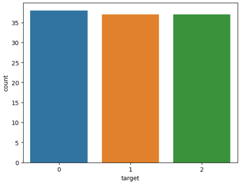
x_train, x_valid, y_train, y_valid = train_test_split(df_iris.drop('target', 1), df_iris['target'], stratify=df_iris['target'])
stratify에 target 데이터를 넣어주게 되면 클래스의 분포를 균등하게 배분할 수가 있다.
sns.countplot(x=y_train)
로지스틱 회귀(Logistic Regression)
로지스틱 회귀는 “예” 또는 “아니오” 처럼 두 가지로 분류되는 문제를 다루는 데 사용이 된다. 0과 1 사이 값으로 예측을 수행하는 것으로 즉, “예”일 확률과 “아니오”일 확률을 나타내는 것이다.
하지만 3개 이상의 클래스에 대한 판별을 위해서는 다음 전략이 필요하다.
- one-vs-rest(OvR): 각 클래스마다 하나의 이진 분류 모델을 만들어 해당 클래스와 나머지 클래스를 구분
- one-vs-one(OvO): 각 클래쓰 쌍마다 이진 분류 모델을 만들고 각 이진 분류 모델의 예측 결과를 투표하여 가장 많은 투표를 받은 클래스를 선택
LogisticRegression 모델 로드
from sklearn.linear_model import LogisticRegression
모델 선언
model = LogisticRegression()
모델 학습
model.fit(x_train, y_train)
예측
prediction = model.predict(x_valid)
SGDClassifier
SGD(Stochastic Gradient Descent)란 확률적 경사 하강법으로 학습 데이터셋에서 무작위 한 개의 샘플 데이터셋을 추출해 그 샘플에 대해서만 기울기를 계산하는 방법이다. 이를 통해 손실을 최소화하는 가중치를 찾을 수 있다.
SGDClassifier 모델 로드
from sklearn.linear_model import SGDClassifier
모델 선언
sgd = SGDClassifier(random_state=0)
모델 학습
sgd.fit(x_train, y_train)
예측
prediction = sgd.predict(x_valid)
평가
(prediction == y_valid).mean()
하이퍼파라미터
sgd.get_params()
위 명령어를 실행하게 되면 설정된 파라미터들을 확인할 수가 있는데 이 파라미터들을 하이퍼파라미터라고 한다. 하이퍼파라미터 값들을 조절하면서 모델의 성능을 바꾸고 향상시킬 수 있는 것이다.
주요 하이퍼파라미터
sgd = SGDClassifier(penalty='elasticnet', random_state=0, n_jobs=-1)
- penalty: 과적합이 되지 않도록 규제 설정
- random_state: 다른 하이퍼파라미터 값을 변경 했을 때 모델의 성능이 하이퍼파라미터 값의 변경 때문인지 랜덤한 데이터 때문인지 알 수가 없기 때문에 이 값을 고정
- n_jobs: 학습에 사용할 CPU 개수를 지정하는 것으로
-1값은 모두 사용한다는 것을 의미
[참조] 패스트캠퍼스 - 직장인을 위한 파이썬 데이터분석 올인원 패키지 Online.
끝!