회귀(Regression) - 규제
[참조] 패스트캠퍼스 - 직장인을 위한 파이썬 데이터분석 올인원 패키지 Online.
규제(Regularization)
규제란 학습이 과대적합 되는 것을 방지하고자 일종의 penalty를 부여하는 것을 말한다.
- L2 규제(L2 Regularization)
- 각 가중치 제곱의 합에 규제 강도(Regularization Strength) λ를 곱함
- λ를 크게하면 가중치 감소(규제 중시)
- λ를 작게하면 가중치 증가(규제 중시 X)
- L1 규제(L1 Regularization)
- 가중치 합에 규제 강도 λ를 곱해 오차에 더함
- 어떤 가중치(w)는 0이 되어 모델에서 제외되는 특성이 생길 수가 있음
L1 규제는 모델에서 제외되는 특성이 있어 L2 규제가 더 안정적이라 더 많이 사용된다.
릿지(Ridge)
L2 규제를 사용한 모델이 릿지 모델이다. \[Error=MSE+αw^2\]
릿지 모델 로드
from sklearn.linear_model import Ridge
규제를 위한 값
alphas = [100, 10, 1, 0.1, 0.01, 0.001, 0.0001]
- 값이 커질수록 규제가 커짐
릿지 모델 구현 및 시각화
for alpha in alphas:
    ridge = Ridge(alpha=alpha)
    ridge.fit(x_train, y_train)
    pred = ridge.predict(x_test)
    mse_eval('Ridge(alpha={})'.format(alpha), pred, y_test)
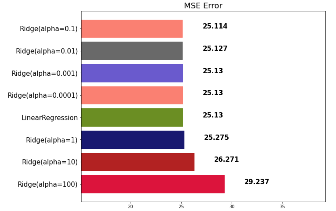
이처럼 α 값에 따른 MSE 수치를 확인할 수가 있다.
릿지 모델 가중치(coefficient) 확인
def plot_coef(columns, coef):
    coef_df = pd.DataFrame(list(zip(columns, coef)))
    coef_df.columns=['feature', 'coef']
    coef_df = coef_df.sort_values('coef', ascending=False).reset_index(drop=True)

    fig, ax = plt.subplots(figsize=(9, 7))
    ax.barh(np.arange(len(coef_df)), coef_df['coef'])
    idx = np.arange(len(coef_df))
    ax.set_yticks(idx)
    ax.set_yticklabels(coef_df['feature'])
    fig.tight_layout()
    plt.show()
위 함수를 이용해 α 값을 다르게 했을 때 coef를 확인해 보도록 한다.
ridge_100 = Ridge(alpha=100)
ridge_100.fit(x_train, y_train)
ridge_pred_100 = ridge_100.predict(x_test)

ridge_001 = Ridge(alpha=0.001)
ridge_001.fit(x_train, y_train)
ridge_pred_001 = ridge_001.predict(x_test)
α = 100
plot_coef(x_train.columns, ridge_100.coef_)
α = 0.001
plot_coef(x_train.columns, ridge_001.coef_)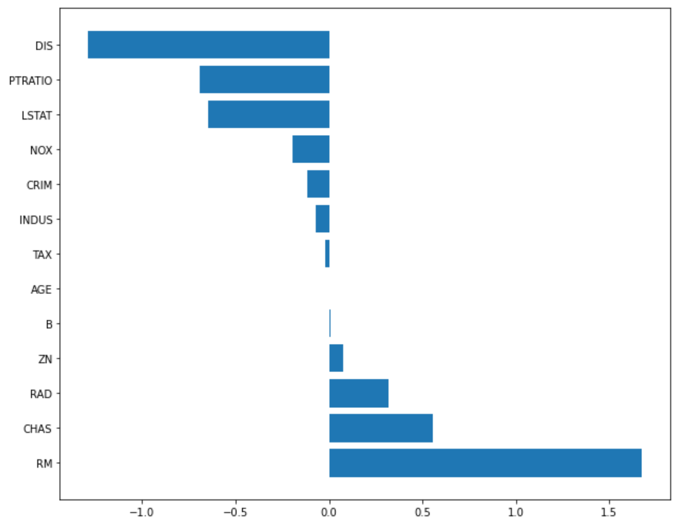
라쏘(Lasso)
L1 규제를 사용한 모델이 라쏘 모델이다. \[Error=MSE+α|w|\]
라쏘 모델 로드
from sklearn.linear_model import Lasso
규제를 위한 값
alphas = [100, 10, 1, 0.1, 0.01, 0.001, 0.0001]
- 값이 커질수록 규제가 커짐
라쏘 모델 구현 및 시각화
for alpha in alphas:
    lasso = Lasso(alpha=alpha)
    lasso.fit(x_train, y_train)
    pred = lasso.predict(x_test)
    mse_eval('Lasso(alpha={})'.format(alpha), pred, y_test)
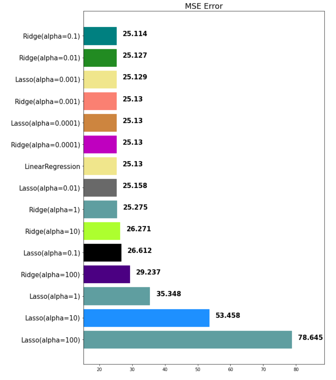
이처럼 α 값에 따른 MSE 수치를 확인할 수가 있다.
라쏘 모델 가중치(coefficient) 확인
위 plot_coef() 함수를 이용해 α 값을 다르게 했을 때 coef를 확인해 보도록 한다.
lasso_100 = Lasso(alpha=100)
lasso_100.fit(x_train, y_train)
lasso_pred_100 = lasso_100.predict(x_test)

lasso_001 = Lasso(alpha=0.001)
lasso_001.fit(x_train, y_train)
lasso_pred_001 = lasso_001.predict(x_test)
α = 100
plot_coef(x_train.columns, lasso_100.coef_)
α = 0.001
plot_coef(x_train.columns, lasso_001.coef_)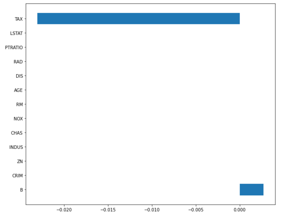
엘라스틱넷(ElasticNet)
엘라스틱넷은 릿지모델과 라쏘모델을 섞은 하이브리트 형태의 모델을 말한다.
l1_ratio
- l1_ratio = 0: L2 규제만 사용
- l1_ratio = 1: L1 규제만 사용
- 0 < l1_ratio < 1: L1, L2 규제 혼합 사용
- default 값은 0.5
엘라스틱넷 모델 로드
from sklearn.linear_model import ElasticNet
ratio 값
ratios = [0.2, 0.5, 0.8]
- 값이 커질수록 규제가 커짐
엘라스틱넷 모델 구현 및 시각화
for ratio in ratios:
    elasticnet = ElasticNet(alpha=0.5, l1_ratio=ratio)
    elasticnet.fit(x_train, y_train)
    pred = elasticnet.predict(x_test)
    mse_eval('ElasticNet(l1_ratio={})'.format(ratio), pred, y_test)
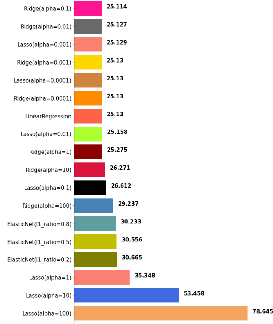
이처럼 α 값에 따른 MSE 수치를 확인할 수가 있다.
엘라스틱넷 모델 가중치(coefficient) 확인
위 plot_coef() 함수를 이용해 α 값은 고정, l1_ratio 값을 다르게 했을 때 coef를 확인해 보도록 한다.
elsticnet_20 = ElasticNet(alpha=5, l1_ratio=0.2)
elsticnet_20.fit(x_train, y_train)
elasticnet_pred_20 = elsticnet_20.predict(x_test)

elsticnet_80 = ElasticNet(alpha=5, l1_ratio=0.8)
elsticnet_80.fit(x_train, y_train)
elasticnet_pred_80 = elsticnet_80.predict(x_test)
l1_ratio = 0.2
plot_coef(x_train.columns, lasso_100.coef_)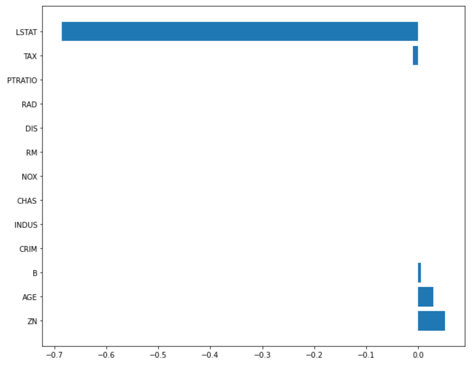
l1_ratio = 0.8
plot_coef(x_train.columns, lasso_001.coef_)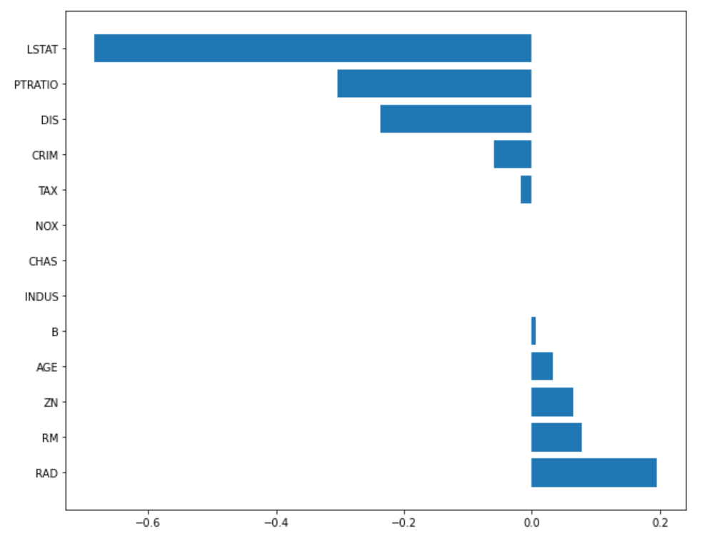
[참조] 패스트캠퍼스 - 직장인을 위한 파이썬 데이터분석 올인원 패키지 Online.
끝!